Chapter 2 Fields and Vector Spaces

2.1 Fields

Definition 2.1 A field is a set $F$ together with binary operations on $F$, which we will refer to as addition and multiplication, such that:

$F$ together with addition is an abelian group (we use the notation $a+b$, $0$ or $0_F$, $-a$), and
$F^{\times} := F \setminus \{0\}$ together with multiplication is an abelian group (we use the notation $a\cdot b$ or $ab$, $1$, $a^{-1}$),

and such that the following axiom holds:
Distributivity: For all $a,b,c \in F$ we have $a(b+c) = ab + ac$ in $F$.

Example 2.2

The sets $\mathbb{Q}, \mathbb{R}$ and $\mathbb{C}$ with the usual addition and multiplication are fields (see also 1.2(b)).
The set $\mathbb{Z}$ with the usual addition and multiplication is not a field because for instance there is no multiplicative inverse of 2 in $\mathbb{Z}$.
The set $\mathbb{F}_{2} := \{ 0, 1 \}$ together with the following operations is a field. \[ \begin{array}{c|cc} {+} & 0 & 1 \\ \hline 0 & 0 & 1 \\ 1 & 1 & 0 \end{array} \qquad \qquad \qquad \begin{array}{c|cc} \cdot & 0 & 1 \\ \hline 0 & 0 & 0 \\ 1 & 0 & 1 \end{array} \] Note that $1 + 1 = 2$ in $\mathbb{Q}$ but $1 + 1 =0$ in $\mathbb{F}_{2}$. $\mathbb{F}_{2}$ is the smallest field.

Proof (that $\mathbb{F}_2$ is a field): $\mathbb{F}_{2}$ with “$+$”, and $\mathbb{F}_{2} \setminus \{ 0 \} = \{1\}$ with “$\cdot$”, are abelian groups (see 1.5(a)).
  Distributivity: We need to check $a(b+c) = ab + ac$ for all $a, b, c \in \mathbb{F}_{2}$.
    First case: $a=0 \implies$ LHS $=0$, RHS $= 0+0 =0$.
    Second case: $a=1 \implies$ LHS $= b+c =$ RHS. $\square$

(without proof) Let $p$ be a prime. The set $\mathbb{F}_p$ $:= \{ \overline{0}, \overline{1}, \dots , \overline{p-1} \}$ together with the addition defined in Example 1.5(b) and the following multiplication is a field: \[ \overline{x} \cdot \overline{y} := \overline{\text{remainder left when $xy$ is divided by $p$}}. \] (Why does this not work when $p$ is not a prime, e.g. if $p=4$?)

Proposition 2.3 Let $F$ be a field. Then:

For all $a\in F$ we have $0a = 0$.
For all $a,b\in F$ we have $(-a)b = -(ab)$.

Proof. (a) We have $0 + 0a = 0a = (0 + 0)a = 0a + 0a$ ($0$ is neutral for “$+$” and by distributivity)
$\implies 0 = 0a$. (cancel $0a$ on both sides using 1.4(a))

We have $ab + (-a)b = (a + (-a))b$ (by distributivity)
$= 0b$ (by definition of the additive inverse)
$= 0$ (by part (a))
$\implies (-a)b$ is the additive inverse of $ab$, i.e. $(-a)b = -(ab)$. $\square$

2.2 Vector spaces

Definition 2.4 Let $F$ be a field. A vector space over $F$ is an abelian group $V$ (we will use “$+$” for the binary operation) together with a map $F \times V \to V$ (called scalar multiplication and written as $(a,x) \mapsto ax$), such that the following axioms are satisfied:

$1^{st}$ distributivity law: For all $a,b \in F$ and $x \in V$ we have $(a + b)x = ax + bx$ in $V$.
$2^{nd}$ distributivity law: For all $a\in F$ and $x,y \in V$ we have $a(x + y) = ax + ay$ in $V$.
For all $a, b \in F$ and for all $x \in V$ we have $(ab)x = a(bx)$ in $V$.
For all $x \in V$ we have $1x = x$ in $V$.

The elements of $V$ are called vectors. The elements of $F$ will be referred to as scalars. We write $0_F$ and $0_{V}$ for the neutral elements of $F$ and $V$, respectively, and often just $0$ for both (when it is clear from the context if it is a scalar or a vector). Furthermore we use the notation $u-v$ for $u + (-v)$ when $u,v$ are both vectors, or both scalars.

Example 2.5

For every $n \in \mathbb{N}$ the set $\mathbb{R}^{n}$ together with the usual addition and scalar multiplication (as seen in Linear Algebra I) is a vector space over $\mathbb{R}$. Similarly, for any field $F$, the set \[ {\color{red}{F^n}} := \{ (a_{1}, \dots ,a_{n}) : \ a_{1}, \dots ,a_{n} \in F \} \] together with component-wise addition and the obvious scalar multiplication is a vector space over $F$. For example $\mathbb{F}_{2}^{2} = \{ (0,0),(0,1),(1,0),(1,1) \}$ is a vector space over $\mathbb{F}_{2}$; $F=F^{1}$ is a vector space over $F$, and finally $F^0:=\{ 0 \}$ is a vector space over $F$.
Let $V$ be the additive group of $\mathbb{C}$. We view the usual multiplication $\mathbb{R} \times V \to V, \ (a,x) \mapsto ax$, as scalar multiplication of $\mathbb{R}$ on $V$. Then $V$ is a vector space over $\mathbb{R}$. Similarly, we can think of $\mathbb{C}$ or $\mathbb{R}$ as vector spaces over $\mathbb{Q}$.
Let $V$ denote the abelian group $\mathbb{R}$ (with the usual addition). For $a \in \mathbb{R}$ and $x \in V$ we put $a \otimes x := a^{2}x \in V$; this defines a scalar multiplication \[ \mathbb{R} \times V \to V,\quad (a,x) \mapsto a \otimes x, \] of the field $\mathbb{R}$ on $V$. Which of the vector space axioms (see 2.4) hold for $V$ with this scalar multiplication?

Solution:

We need to check whether $(a+b) \otimes x = a \otimes x + b \otimes x$ for all $a,b \in \mathbb{R}$ and $x \in V$.
LHS $= (a+b)^{2} x$; RHS $= a^{2}x + b^{2}x = (a^{2} + b^{2})x$
$\implies$ For $a=1, b=1$ and $x=1$ we have LHS $\neq$ RHS.
$\implies$ First distributivity law does not hold.
We need to check whether $a \otimes (x + y) = a \otimes x + a \otimes y$ for all $a \in \mathbb{R}$ and $x,y \in V$.
$\left. \begin{aligned} \text{LHS} & = a^{2}(x+y) \\ \text{RHS} & = a^{2}x + a^{2}y = a^{2}(x+y) \end{aligned} \right\} \implies \text{LHS} = \text{RHS}$
$\implies$ Second distributivity law does hold.
We need to check whether $a \otimes (b \otimes x) = (ab) \otimes x$ for all $a,b \in \mathbb{R}$ and $x \in V$.
$\left. \begin{aligned} \text{LHS} & = a \otimes (b^{2}x) = a^{2} (b^{2}x) \\ \text{RHS} & = (ab)^{2}x = (a^{2}b^{2})x = a^{2} (b^{2}x) \end{aligned} \right\} \implies \text{LHS} = \text{RHS}$
$\implies$ Axiom (iii) does hold.
We have $1 \otimes x = 1^{2} x = x$ for all $x \in V$.
$\implies$ Axiom (iv) does hold.

Proposition 2.6 Let $V$ be a vector space over a field $F$ and let $a,b \in F$ and $x,y \in V$. Then we have:

$(a-b)x = ax - bx$
$a(x-y) = ax - ay$
$ax = 0_{V} \iff a = 0_{F}$ or $x=0_{V}$
$(-1)x = -x$

Proof: (a) $(a-b)x + bx = ((a-b)+b)x$ (by first distributivity law)
$= \left(a+((-b)+b)\right)x=(a+0_F)x = ax$ (using field axioms)
$\implies (a-b)x = ax - bx$. (add $-bx$ to both sides)

On Coursework.
“$\Longrightarrow$”: On Coursework.
“$\Longleftarrow$”: Put $a=b$ and $x=y$ in (a) and (b), respectively.
Put $a=0$ and $b=1$ in (a) and use (c). $\square$

The next example is the “mother” of almost all vector spaces. It vastly generalises the fourth of the following five ways of representing vectors and vector addition in $\mathbb{R}^{3}$.

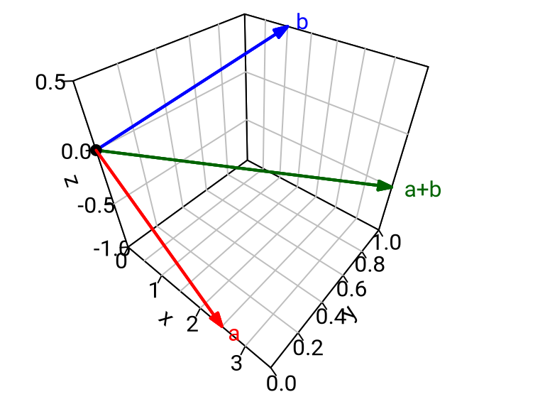
${\color{red}{\underline{a} = (2.5,0,-1)}} \qquad {\color{blue}{\underline{b} = (1,1,0.5)}} \qquad {\color{green}{\underline{a}+\underline{b} = (3.5,1,-0.5)}}$
${\color{red}{\underline{a} = \begin{pmatrix} 1 & 2 & 3 \\ 2.5 & 0 & -1 \end{pmatrix}}} \qquad {\color{blue}{\underline{b} = \begin{pmatrix} 1 & 2 & 3 \\ 1 & 1 & 0.5 \end{pmatrix}}} \qquad {\color{green}{\underline{a}+\underline{b} = \begin{pmatrix} 1 & 2 & 3 \\ 3.5 & 1 & -0.5 \end{pmatrix}}}$
$\begin{aligned} {\color{red}{\underline{a}: \{ 1,2,3}} & {\color{red}{\} \to \mathbb{R}}} & \quad {\color{blue}{\underline{b}: \{ 1,2,3}} & {\color{blue}{\} \to \mathbb{R}}} & \quad {\color{green}{\underline{a}+\underline{b}: \{ 1,2,3}} & {\color{green}{\} \to \mathbb{R}}} \\ & {\color{red}{1 \mapsto 2.5}} & & {\color{blue}{1 \mapsto 1}} & & {\color{green}{1 \mapsto 3.5}} \\ & {\color{red}{2 \mapsto 0}} & & {\color{blue}{2 \mapsto 1}} & & {\color{green}{2 \mapsto 1}} \\ & {\color{red}{3 \mapsto -1}} & & {\color{blue}{3 \mapsto 0.5}} & & {\color{green}{3 \mapsto -0.5}} \end{aligned}$

Example 2.7 Let $S$ be any set and let $F$ be a field. Let \[ {\color{red}{F^S}} := \{ f: S \to F \} \] denote the set of all maps from $S$ to $F$. We define an addition on $F^{S}$ and a scalar multiplication of $F$ on $F^{S}$ as follows: When $f,g \in F^{S}$ and $a \in F$ we set: \[ \begin{aligned} ({\color{red}{f+g}})(s) & := f(s) + g(s) \qquad & \text{for any } s \in S \\ ({\color{red}{af}})(s) & := af(s) & \text{for any } s \in S. \end{aligned} \] Then $F^{S}$ is a vector space over $F$ (see below for the proof).

Special Cases:

Let $S = \{1,\dots,n\}$. Identifying any map $f: \{1,\dots,n\} \to F$ with the corresponding tuple $(f(1),\dots,f(n))$, we see that $F^{S}$ can be identified with the set $F^{n}$ of all $n$-tuples $(a_{1},\dots,a_{n})$ considered in Example 2.5(a).
Let $S = \{1,\dots,n\} \times \{1,\dots,m\}$. Identifying any map $f: \{1,\dots,n\} \times \{1,\dots,m\} \to F$ with the corresponding matrix: \[ \begin{pmatrix} f((1,1)) & \dots & f((1,m)) \\ \vdots & & \vdots \\ f((n,1)) & \dots & f((n,m)) \end{pmatrix} \] we see that $F^{S}$ can be identified with the set $M_{n \times m}(F)$ of $(n \times m)$-matrices \[ \begin{pmatrix} a_{11} & \dots & a_{1m} \\ \vdots & \ddots & \vdots \\ a_{n1} & \dots & a_{nm} \end{pmatrix} \] with entries in $F$. In particular $M_{n \times m}(F)$ is a vector space over $F$.
Let $S = \mathbb{N}$. Identifying any map $f: \mathbb{N} \to F$ with the sequence $(f(1), f(2), f(3), \dots)$ we see that $F^{\mathbb{N}}$ can be identified with the set of all infinite sequences $(a_{1},a_{2},a_{3}, \dots)$ in $F$.
Let $F=\mathbb{R}$ and let $S$ be an interval $I$ in $\mathbb{R}$. Then $F^{S}=\mathbb{R}^I$ is the set of all functions $f: I \to \mathbb{R}$. (We can visualise these functions via their graph, similarly as in (V) above.)

Proof (that $F^S$ is a vector space over $F$): First, $F^S$ with the above defined “$+$” is an abelian group:

Associativity: Let $f,g,h \in F^{S}$.
We need to show: $(f+g)+h = f+(g+h) \text{ in } F^{S}$
$\iff ((f+g)+h)(s) = (f+(g+h))(s) \qquad$ for all $s \in S$.
$\left. \begin{aligned} \text{LHS} = (f+g)(s) + h(s) & = (f(s) + g(s)) + h(s) \\ \text{RHS} = f(s) + (g+h)(s) & = f(s) +(g(s) + h(s) \end{aligned} \right\}$ (by definition of addition in $F^{S}$)
$\implies$ LHS = RHS (by associativity in $F$)

Identity element: Let $\underline{0}$ denote the constant function $S \to F, s \mapsto 0_{F}$.
For any $f \in F^{S}$ and $s\in S$ we have $(f + \underline{0})(s) = f(s) + \underline{0}(s) = f(s) + 0_{F} = f(s)$, hence $f + \underline{0} = f$.
Similarly we have $\underline{0} + f = f$. (using definitions of $\underline{0}$ and “$+$”, and field axioms)
$\implies \underline{0}$ is the identity element.

Inverses: Let $f \in F^{S}$. Define $(-f)(s) := -f(s)$.
For any $s\in S$ we have $(f+(-f))(s) = f(s) + (-f)(s) = f(s) + (-f(s)) = 0_F = \underline{0}(s)$.
$\implies f + (-f) = \underline{0}$ in $F^{S}$, so $-f$ is the inverse to $f$. ($\uparrow$ defns of “$+$”, “$-f$”, $\underline{0}$, and field axioms)

Commutativity: Let $f,g\in F^S$.
For any $s\in S$ we have $(f+g)(s)=f(s)+g(s) = g(s) + f(s) = (g+f)(s)$.
$\implies f+g=g+f$. ($\uparrow$ by the definition of “$+$”, and commutativity of $+$ in $F$)

Now the four axioms from Definition 2.4 (only (i) and (iii) spelled out here, the others are similar):

First distributivity law: Let $a,b \in F$ and $f \in F^{S}$. We want to check that $(a+b)f = af + bf$:
For all $s \in S$ we have
$((a+b)f)(s) = (a+b)(f(s))$ (by definition of the scalar multiplication)
     $= a(f(s)) + b(f(s))$ (by distributivity in $F$)
     $= (af)(s) + (bf)(s)$ (by definition of the scalar multiplication)
     $= (af + bf)(s)$ (by definition of addition in $F^{S}$)
$\implies (a+b)f = af + bf$.

Axiom (iii): Let $a,b\in F$ and $f\in F^S$. We want to check that $(ab)f = a(bf)$.
For all $s\in S$ we have
$((ab)f)(s) = (ab)(f(s))$ (by definition of scalar multiplication in $F^S$)
     $=a(b(f(s)))$ (by associativity of multiplication in $F$)
     $=a((bf)(s))$ (by definition of scalar multiplication in $F^S$)
     $=(a(bf))(s)$ (by definition of scalar multiplication in $F^S$)
$\implies$ $(ab)f = a(bf)$. $\square$

2.3 Subspaces

Definition 2.8 Let $V$ be a vector space over a field $F$. A subset $W$ of $V$ is called a subspace of $V$ if the following conditions hold:

$0_{V} \in W$.
“$W$ is closed under addition”: for all $x,y \in W$ we also have $x+y \in W$.
“$W$ is closed under scalar multiplication”: for all $a \in F$ and $x \in W$ we have $ax \in W$.

Note that condition (b) states that the restriction of the addition in $V$ to $W$ gives a binary operation $W \times W \to W$ on $W$ (addition in $W$). Similarly, condition (c) states that the scalar multiplication of $F$ on $V$ yields a map $F \times W \to W$ which we view as a scalar multiplication of $F$ on $W$.

Proposition 2.9 Let $V$ be a vector space over a field $F$ and let $W$ be a subspace of $V$. Then $W$ together with the above mentioned addition and scalar multiplication is a vector space over $F$.

Proof: The following axioms hold for $W$ because they already hold for $V$:

associativity of addition;
commutativity of addition;
all the four axioms in Definition 2.4.

There exists an additive identity element in $W$ by condition 2.8(a) (i.e. $0_W:=0_V\in W$).
It remains to show that additive inverses exist: Let $x \in W$. Then $-x = (-1)x$ (see 2.6(d)) is in $W$ by condition 2.8(c); and $-x$ satisfies $x+(-x) = 0_W=0_V$ because it does so in $V$. $\square$

Example 2.10

Examples of subspaces of $\mathbb{R}^{n}$ as seen in Linear Algebra I, such as the nullspace of any real $(n \times m)$-matrix, or the column space of any real $(m\times n)$-matrix.
The set of convergent sequences is a subspace of the vector space $\mathbb{R}^{\mathbb{N}}$ of all sequences $(a_{1},a_{2},a_{3}, \dots)$ in $\mathbb{R}$. A subspace of this subspace (and hence of $\mathbb{R}^{\mathbb{N}}$) is the set of all sequences in $\mathbb{R}$ that converge to $0$. (See Calculus I for proofs).
Let $A \in M_{l \times m}(\mathbb{R})$. Then $W := \{B \in M_{m \times n}(\mathbb{R}) \mid AB = \underline{0} \}$ is a subspace of $M_{m \times n}(\mathbb{R})$.
Proof:
1. We have $A \cdot \underline{0} = \underline{0} \implies \underline{0} \in W$.
2. Let $B_{1},B_{2} \in W$
  $\implies A(B_{1} + B_{2}) = AB_{1} + AB_{2} = \underline{0} + \underline{0} = \underline{0}$
  $\implies B_{1} + B_{2} \in W$.
3. Let $a \in \mathbb{R}$ and $B \in W$
  $\implies A(aB) = a(AB) = a \underline{0} = \underline{0}$
  $\implies aB \in W$. $\square$
Let $I$ be a non-empty interval in $\mathbb{R}$. The following subsets of the vector space $\mathbb{R}^{I}$ consisting of all functions from $I$ to $\mathbb{R}$ are subspaces:
1. For any $s_{0} \in I$ the subset $W := \{ f \in \mathbb{R}^{I} : f(s_{0})=0 \}$ of $\mathbb{R}^{I}$.
  Proof:
  1. The zero function $\underline{0}$ vanishes at $s_{0} \implies \underline{0} \in W$.
  2. Let $f,g \in W$
    $\implies (f+g)(s_{0}) = f(s_{0}) + g(s_{0}) = 0 + 0 = 0$
    $\implies f+g \in W$.
  3. Let $a \in \mathbb{R}$ and $f \in W$
    $\implies (af)(s_{0}) = a\cdot f(s_{0}) = a\cdot 0 = 0$
    $\implies af \in W$. $\square$
2. The set of all continuous functions $f: I \to \mathbb{R}$ (see Calculus I).
3. The set of all differentiable functions $f: I \to \mathbb{R}$ (see Calculus I).
4. For any $n \in \mathbb{N}$, the set $\mathbb{P}_n$ of polynomial functions $f: I \to \mathbb{R}$ of degree at most $n$, is a subspace by 3.2(c) and 3.3. A function $f: I \to \mathbb{R}$ is a polynomial function of degree at most $n$ if there exists $a_{0}, \dots ,a_{n} \in \mathbb{R}$ such that: \[ f(s) = a_{0} + a_{1}s + \dots + a_{n}s^{n} \text{ for all } s \in I. \] Denoting the function $I \to \mathbb{R}, s \mapsto s^{m}$, by $t^m$, this means that $f = a_{0}t^0 + a_{1}t^1 + \dots + a_{n}t^{n}$ as elements of the vector space $\mathbb{R}^{I}$. (We will also use the more natural notation $1$ for $t^0$, and $t$ for $t^1$.)
5. The space of solutions of a homogeneous linear differential equation (without further explanation); e.g.: \[ \mathbb{P}_{n} = \{ f \in \mathbb{R}^{I} : f \text{ is differentiable } (n+1) \text{ times and } f^{(n+1)} = \underline{0} \} \]
The subset $\mathbb{Z}^{n}$ of the vector space $\mathbb{R}^{n}$ over $\mathbb{R}$ is closed under addition but not closed under scalar multiplication: For instance, $(1,0, \dots ,0) \in \mathbb{Z}^{n}$ and $\frac{1}{2} \in \mathbb{R}$, but $\frac{1}{2}(1,0, \dots ,0) \notin \mathbb{Z}^{n}$.
The subsets $W_{1} := \{ (a,0) : a \in \mathbb{R} \}$ and $W_{2} := \{ (0,b) : b \in \mathbb{R} \}$ are subspaces of $\mathbb{R}^{2}$. The subset $W := W_{1} \cup W_{2}$ of the vector space $\mathbb{R}^{2}$ is closed under scalar multiplication but not under addition because, for instance, $(1,0)$ and $(0,1)$ are in $W$ but $(1,0) + (0,1) = (1,1) \notin W$.

Proposition 2.11 Let $W_{1},W_{2}$ be subspaces of a vector space $V$ over a field $F$. Then the intersection $W_{1} \cap W_{2}$ and the sum of subspaces \[ {\color{red}{W_{1} + W_{2}}} := \{ x_{1} + x_{2}\in V \mid x_{1} \in W_{1}, \ x_{2} \in W_{2} \} \] are subspaces of $V$ as well.

Proof: For $W_{1} \cap W_{2}$:

We have $0_V\in W_1$ and $0_V\in W_2$ (because $W_1$ and $W_2$ are subspaces)
$\implies$ $0_V\in W_1\cap W_2$. (by definition of intersection)
Let $x,y\in W_1\cap W_2$
$\implies$ $x,y \in W_1$ and $x,y\in W_2$ (by definition of intersection)
$\implies$ $x+y\in W_1$ and $x+y\in W_2$ (because $W_1$ and $W_2$ are subspaces)
$\implies$ $x+y\in W_1\cap W_2$. (by definition of intersection)
Let $a\in F$ and $x\in W_1\cap W_2$
$\implies$ $x \in W_1$ and $x\in W_2$ (by definition of intersection)
$\implies$ $ax\in W_1$ and $ax\in W_2$ (because $W_1$ and $W_2$ are subspaces)
$\implies$ $ax\in W_1\cap W_2$. (by definition of intersection)

For $W_{1} + W_{2}$:

We have $0_{V} = 0_{V} + 0_{V} \in W_{1} + W_{2}$.
Let $x,y \in W_{1} + W_{2}$
$\implies \exists x_{1},y_{1} \in W_{1}$ and $\exists x_{2},y_{2} \in W_{2}$ with $x=x_{1}+x_{2}$, $y=y_{1}+y_{2}$ (by definition of $W_1+W_2$)
$\implies x + y = (x_{1}+x_{2}) + (y_{1}+y_{2}) =$
$=(x_{1}+y_{1}) + (x_{2}+y_{2}) \in W_{1} + W_{2}$. (because $W_{1}$ and $W_{2}$ are subspaces)
Let $a \in F$ and $x \in W_{1} + W_{2}$
$\implies \exists x_{1} \in W_{1}$, $x_{2} \in W_{2}$ such that $x=x_{1}+x_{2}$ (by definition of $W_1+W_2$)
$\implies ax = a (x_{1}+x_{2}) = ax_{1} + ax_{2} \in W_{1} + W_{2}$. (because $W_{1}$ and $W_{2}$ are subspaces)$\square$

Example 2.12 Let $W_{1}$ and $W_{2}$ be as in 2.10(f). Then $W_{1} + W_{2} = \mathbb{R}^{2}$.